5 posts tagged with "BigQuery"

View All Tags

Introducing Starlake.ai

· 2 min read
Abdelhamide El Arib
Starlake Core Team

We're excited to unveil Starlake.ai, a groundbreaking platform designed to streamline your data workflows and unlock the full potential of your data. 🚀

The Challenges We Solve

In the modern data landscape, businesses often face these challenges:

  • Overwhelming complexity in managing data pipelines
  • Inefficiencies in transforming and orchestrating data workflows
  • Lack of robust governance and data quality assurance

Starlake tackles these problems head-on, offering a declarative data pipeline solution that simplifies the entire data lifecycle.
Our Mission

  1. Simplify Data Management: Automate ingestion, transformation, and orchestration to reduce manual effort.
  2. Enhance Data Quality: Enforce schema validation, governance rules, and SLA tracking to ensure data consistency.
  3. Accelerate Insights: Deliver clean, transformed, and analytics-ready data faster and more reliably.

Core Capabilities

  • No-Code Data Ingestion: Seamlessly ingest and validate data from any source—no coding required.
  • Low-Code Transformations: Use YAML and SQL to apply transformation rules at scale.
  • Automated Workflow Orchestration: Simplify dependencies with Airflow and Dagster integrations.
  • Data Governance and Quality: Ensure schema enforcement, validation, and SLA tracking.
  • Multi-Cloud and On-Prem Support: Run on your preferred infrastructure, including Snowflake, Databricks, and BigQuery.

Why Starlake Stands Out

Starlake doesn’t just manage your data pipelines—it transforms them. Here’s how we compare:

FeatureStarlake.aiTraditional ETL Tools
No-Code Ingestion
Declarative Transformations
Automated Orchestration
Built-in Governance

Start Your Journey with Starlake

Getting started with Starlake is effortless:

  1. Join the Waitlist: Be among the first to explore Starlake Cloud.
  2. Integrate Your Data Sources: Quickly connect to your preferred databases and warehouses.
  3. Streamline Your Workflows: Start experiencing the power of automated, no-code pipelines.

Ready to Transform Your Data Workflows?

Starlake.ai is here to revolutionize how you manage, transform, and govern your data. Join the movement and discover a smarter way to handle data pipelines.

Learn more at Starlake.ai.

How to Load and Transform into BigQuery Wildcard Tables

· 5 min read
Hayssam Saleh
Starlake Core Team

Sharding

BigQuery Wildcard Tables

When loading files into BigQuery, you may need to split your data into multiple partitions to reduce data size, improve query performance, and lower costs. However, BigQuery’s native partitioning only supports columns with date/time or integer values. While partitioning on string columns isn’t directly supported, BigQuery provides a workaround with wildcard tables, offering nearly identical benefits.

In this example, we demonstrate how Starlake simplifies the process by seamlessly loading your data into wildcard tables.

The Problem

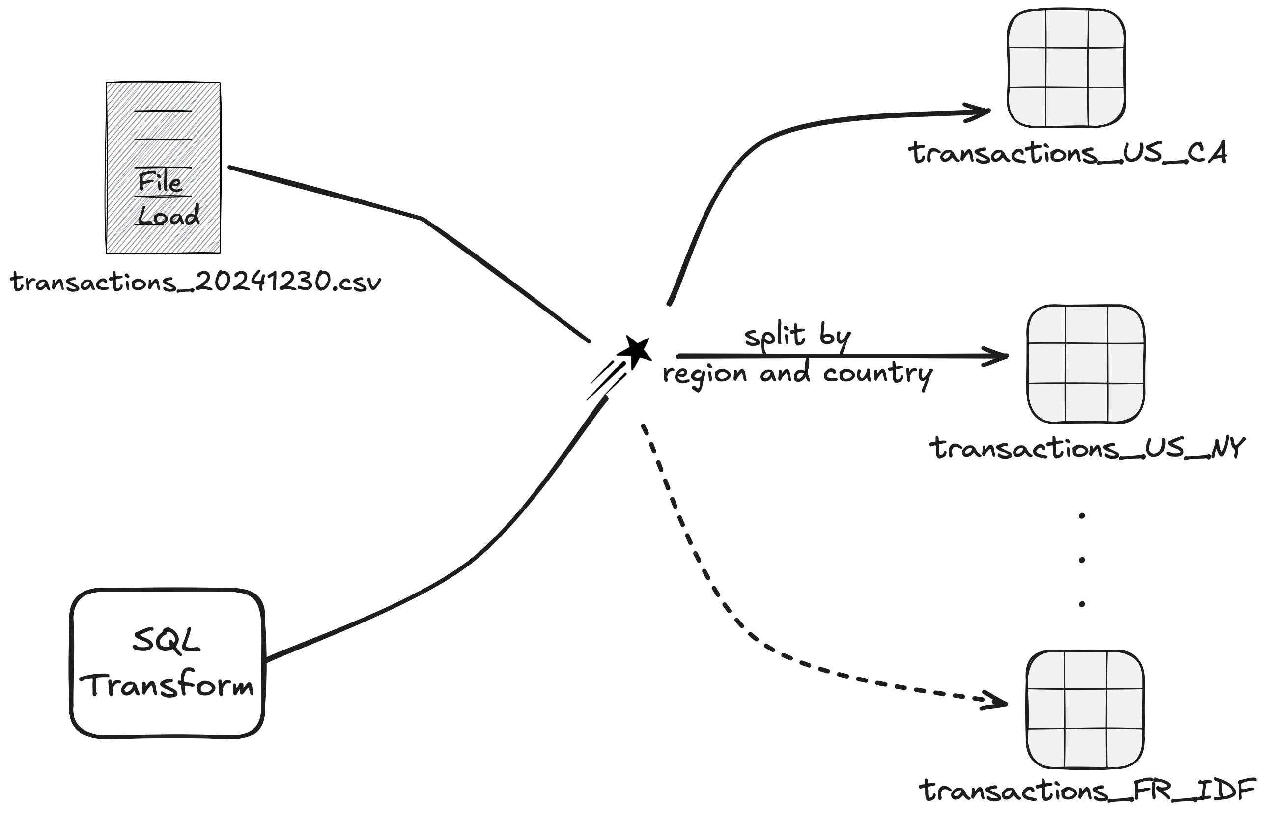
Assume your business receives daily transactions as CSV files from branches across various countries. These files are named in the format transactions_YYYYMMDD.csv, and the goal is to load them into BigQuery, partitioned by country, region and date.

The CSV files contains data in the following format:

store_id, customer_id, trans_id, trans_date, trans_time, country, region, ...
1, 1, 1, 2024-12-19, 12:00:00, US, CA
1, 2, 2, 2024-12-19, 13:01:00, US, CA
2, 3, 3, 2024-12-19, 13:01:00, US, NY
2, 4, 4, 2024-12-19, 13:01:00, US, NY

With hundreds of millions of transactions generated daily, querying the data efficiently by country and region is critical. Partitioning the data in this way would reduce storage size and significantly speed up queries.

However, since BigQuery doesn’t support partitioning by string columns, we can leverage wildcard tables to achieve the same benefits. The desired result is to create separate tables in BigQuery for each country and region, structured as follows:

sales.transactions_US_CA
sales.transactions_US_NY

Each table would store transactions for a specific country and region, while also being partitioned by date for optimal performance.

The Solution with Starlake Load

First, we need to instruct Starlake to infer the schema of the table from the CSV files and load them into BigQuery. This can be achieved with the following command:

starlake infer-schema --domain sales \
--table transactions \
--input transations_20241219.csv

This command infers the schema of the CSV file and generates a YAML file that defines the schema and loading instructions. The resulting YAML file would look like this:

transactions.sl.yml
version: 1
table:
name: "transactions"
pattern: "transations_.*.csv"
attributes:
- name: store_id
type: int
- name: customer_id
type: int
- name: trans_id
type: int
- name: trans_date
type: timestamp
- name: trans_time
type: timestamp
- name: country
type: string
- name: region
type: string
metadata:
format: DSV
withHeader: true
separator: ","
writeStrategy:
type: APPEND

Additionally, a second YAML file specifies where the input files are located:

_config_.sl.yml
version: 1
load:
name: "sales"
metadata:
directory: "{{incoming_path}}/sales"

To load the data into BigQuery, follow these steps:

  1. Place the transaction files, following the expected filename pattern, into the directory {{incoming_path}}/sales. The {{incoming_path}} variable is defined in the environment configuration file.
  2. Run the following command:
starlake load --domain sales --table transactions

Since we aim to partition the data by country, region, and transaction date, and BigQuery does not support string columns for partitioning, we can use wildcard tables to achieve the same benefits.

To implement this, we need to update the metadata section in the transactions.sl.yml file with additional instructions for creating wildcard tables.

transactions.sl.yml
...
metadata:
...
sink:
sharding: [country, region]
partition: [trans_date]

The sharding key tells Starlake to create a wildcard table for each unique combination of country and region. The partition key tells Starlake to partition the data in each wildcard table by transaction date.

We can now load the data into BigQuery and Starlake will create the following tables:

sales.transactions_US_CA
sales.transactions_US_NY

That's it - we've successfully loaded your data into BigQuery using wildcard tables!

Let's query the data to ensure it's been loaded correctly:

SELECT * FROM sales.transactions_*
WHERE _TABLE_SUFFIX = 'US_CA' AND trans_date = '2024-12-19'
SELECT * FROM sales.transactions_*
WHERE _TABLE_SUFFIX in ('US_CA', 'US_NY' ) and trans_date = '2024-12-19'

The Solution with Starlake Transform

In addition to loading data, Starlake also supports transforming data using SQL queries. To create the wildcard tables during the transformation process, We use the exact same attributes in the sink section of the transform YAML file as we did in the load process. Starlake will automatically create the wildcard tables in BigQuery when the transformation is executed.

Conclusion

This section illustrates how Starlake streamlines the process of loading data into BigQuery using wildcard tables.

By leveraging Starlake’s declarative approach, you can effortlessly partition your data by string columns, enhancing query performance while minimizing costs. Additionally, Starlake’s support for both data loading and transformation enables you to seamlessly create wildcard tables as part of the transformation process.

Also, Starlake’s integrated approach ensures consistency by allowing you to reuse the same attributes in the sink section of the transformation YAML file as those defined during the data loading process.

Finally, Starlake’s support for wildcard tables in BigQuery comes with zero additional cost. The data is sharded on the fly at load time in a single step, reducing cost and increasing load & transform jobs performance.

This simplifies workflows and promotes efficiency.

How to unit test your data pipelines

· 6 min read
Bounkong Khamphousone
Starlake Core Team

In today's data-driven landscape, ensuring the reliability and accuracy of your data warehouse is paramount. The cost of not testing your data can be astronomical, leading to critical business decisions based on faulty data and eroding trust. 

The path to rigorous data testing comes with its own set of challenges. In this article, I will highlight how you can confidently deploy your data pipelines by leveraging Starlake JSQLTranspiler and DuckDB, while also reducing costs. we will go beyond testing your transform usually written in SQL and see how we can also test our Ingestion jobs.

The art of mastering data pipelines

Mastering your data pipeline is a challenging art. A data pipeline generally contains the following phases:

  • Collection: Extracting data from sources
  • Ingestion: Loading the extracted data into the data warehouse
  • Transformation: A phase that ultimately adds value to the collected data

The table below summarizes the tests run by Starlake on Load & Transform jobs:

Check to run onIngestion TestTransform Test
Validate the filename pattern
Validate the file structure (number and types of attributes, input file format - CSV / JSON / XML / FIXED-WIDTH)
Check if loaded files or transform SQL SELECT statements  are materialized according to the defined strategy (APPEND / OVERWRITE / UPSERT_BY_KEY, SCD2 …)
Check for missing or unexpected records in the resulting table
Check if the resulting table has a correct schema
Check all expectations
Check time based query output with time freeze
The results of these automated tests are designed for both human review and CI/CD integration. For human review, a website is generated to help users easily identify failures and their causes. For CI/CD integration, a JUnit report is generated, and there is an option to specify a minimum coverage threshold. If the evaluated coverage falls below this threshold, the command will result in an error, and any failing tests will also trigger errors.

Untested SQL costs

Thanks to data pipelines unit testing, we drastically reduce the development cost. Not running tests seems to allow high project's velocity, thereby delivering value quickly. However, the cost of a feature does not stop at its simple development but encompasses all the efforts put in until the feature's completion. Below are some hidden costs.

  • Identifying bugs
    • Without unit tests, verifying development requires deploying the project. This deployment raises challenging questions about the deployment strategy and its rollback or correction procedures.
    • Verification might be carried out by a separate QA team, sometimes even outside the project team. This can lead to the use of feature flags to avoid deploying to production, complicating the implementation. Additionally, waiting for feedback from the QA team introduces delays, increasing the cost of fixing any bugs that arise.
    • Depending on the deployment strategy, verification may also be incomplete due to a lack of control over the test data used.
  • Maintenance and Evolution Complexity
    • Many of us have faced a massive query and struggled to make modifications without disrupting existing functionality, all while aiming for improvements like optimizing processing time. Rigorous unit tests can help with this. They allow us to enhance the expected outcomes in current datasets, create new ones, and compare the modified query results with these expectations. This significantly reduces the risk of regression.
  • Decreased productivity
    • The absence of automated tests often means manually re-running parts or all of the system to ensure correct integration, which can lead to spending time fixing collateral bugs and thus reducing overall productivity. As the project advances, more components need verification, making the process even more time-consuming. This significantly diminishes the willingness to refactor or revise code.
  • Promoting expertise
    • Without unit tests, teams often assign the same tasks to the same people, which hinders skill development and increases the risk of knowledge loss due to turnover.
  • Customer dissatisfaction
    • A project with uncertain product output quality often leads to dissatisfaction, frustration, and a loss of trust in the individual, the team, or the product.

We are all aware of the hidden costs associated with the absence of tests; in my opinion, these are the most significant. Therefore, we will explore how to manage a data pipeline.

Writing unit test in Starlake

Suppose we have the following transform. Starlake transform folder hierachy

We test it by creating the following hierarchy: Starlake test transform folder hierachy

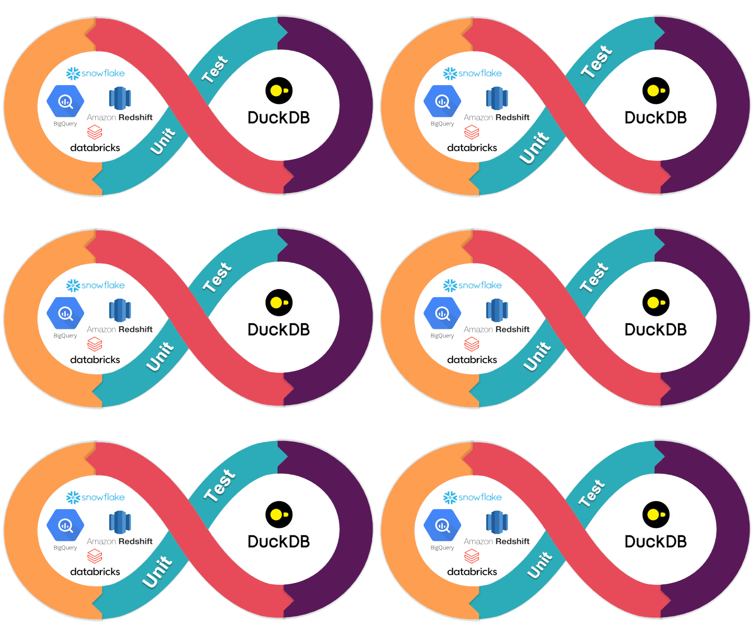
This is then how it is executed Data pipeline unit test lifecycle

Starlake unit tests benefits

Running tests on a local DuckDB database instead of the target Data Warehouse has the following advantages:

  • Fast Feedback: Local execution is significantly faster than using a remote database due to network latency. Additionally, the local environment might be better suited for handling small volumes of test data.
  • No Execution Cost: Depending on the pricing model of the target database, creating temporary resources and executing queries can incur both execution and storage costs.
  • Setup and Cleanup of Automated Tests: Guarantee of resource isolation.
  • Credential Issues: Running tests against a target database requires credentials, which may pose security risks.

Conclusion

In this article, we have demonstrated how adopting unit testing, a crucial practice for software engineers, can significantly enhance the quality of our data pipelines. This approach not only reduces overall costs in the medium to long term but also ensures the maintenance of dynamic and enduring documentation. Additionally, implementing unit tests is essential for rigorous CI/CD processes, enabling seamless continuous data pipeline deployment.

If you encounter any issues while performing your tests locally, please report them on the Starlake GitHub repository. Your feedback is invaluable in improving local test coverage, empowering more data engineers to deploy their work confidently and smoothly. For further discussions and support, join our team on Slack.

We greatly appreciate your contributions. If you found this article helpful, please star the project on GitHub and share it on your social networks to help us reach a broader audience.

Column and Row Level Security in BigQuery

· 3 min read
Hayssam Saleh
Starlake Core Team Member

Data exposition strategies

Data may be exposed using views or authorized views and more recently using Row / Column level security.

Historically, to restrict access on specific columns or rows in BigQuery, one can create a (authorized) view with a SQL request like the one below:

CLS / RLS using Views

BigQuery Views require to grant access for the end users to the table on top of which the view is created. To bypass that limitation, BigQuery provide Authorized views. However, Authorized views come with the following restrictions:

  1. The underlying table is accessed through the authorized view where the end user is impersonated, loosing thus at the table level, the identity of the user making the request. Impersonation

  2. Each restriction policy require to define a specific authorized view making it difficult to identify who has access to what ? Multiplication of Authorized Views

  3. Authorized views need to be updated whenever a schema evolution on the underlying table bring in a sensitive field that need to be excluded or a field that need to be included in the view. In the example below, the new column "description" need to be added to the authorized view if we want it . Multiplication of Authorized Views

That's where Row Level Security and Column Level security features natively supported by BigQuery come in.

BigQuery Row Level Security

Row Level Security restrict access to the rows based on the conditions set in the where clause using the custom SQL statement below:

RLS

Big Query Column Level Security

Column level security in BigQuery is managed using a taxonomy. This taxonomy is a hierarchy of policy tags describing the table attributes or other resources. By assigning access rights to a tag, we restrict access to any resource tagged using this specific tag and this applies to BigQuery table fields.

In our example, restricting access to specific user/group/sa to the column price require the following steps:

  1. In Cloud Data Catalog/Policy Tags, create a Taxonomy. Note that Enfore access control should be checked.

CLS Taxonomy

  1. Assign permissions for each policy tag you defined

CLS Access

  1. Tag restricted columns in the BigQuery schema editor. CLS Assign
tip

Assigning policy tags may be done using the bq load/update command line tool

BigQuery RLS/CLS benefits

Using BigQuery row and column level security features bring several benefits:

  • There is no need to create extra views
  • Users use the same name for the table but with different access rights
  • A company-wide taxonomy is defined allowing better Data Management
  • Access rights to a new column in the table are automatically handled

A word about RLS and CLS in Starlake

Ingesting Data into BigQuery cannot be considered complete without taking into account the access level restrictions on the target table. Starlake will handle for you all the scripting required to secure BigQuery rows and columns using a YAML declarative syntax to make sure that your tables are secured in BigQuery:

Declarative Row Level & Column Level Security
  - name: "PRODUCT"
rls:
- name: "my-rls"
predicate: "category like 'Food'"
grants:
- "user:[email protected]"
- "group:[email protected]"
- "sa:[email protected]"
attributes:
- name: "id"
accessPolicy: PII

Handling Dynamic Partitioning and Merge with Spark on BigQuery

· 7 min read
Hayssam Saleh
Starlake Core Team Member

Data Loading strategies

When loading data into BigQuery, you may want to:

  • Overwrite the existing data and replace it with the incoming data.
  • Append incoming data to existing
  • Dynamic partition Overwrite where only the partitions to which the incoming data belong to are overwritten.
  • Merge incoming data with existing data by keeping the newest version of each record.

For performance reasons, when having huge amount of data, tables are usually split into multiple partitions. BigQuery supports range partitioning which are uncommon and date/time partitioning which is the most widely used type of partitioning. The diagram below shows our initial table partitioned by the date field.

Initial data

Let's assume we receive the following data that we need to ingest into the table:

Incoming data

The strategies above will produce respectively the results below:

The table ends up with the 2 incoming records. All existing partitions are deleted.

Overwrite data

There is no good or bad strategy, the use of one of the strategies above depends on the use case. Some use case examples for each of the strategies are:

  • Overwrite mode may be useful when you receive every day the list of all product names.
  • Append mode may be useful when you receive daily sales.
  • Dynamic Partition Overwrite mode may be useful when you ingested the first time a partition, and you need to ingest it again with a different set of data and thus alter only that partition.
  • Merge mode may be useful when you receive product updates every day and that you need to keep only the last version of each product.

Spark How-to

Apache Spark SQL connector for Google BigQuery makes BigQuery a first class citizen as a source and sink for Spark jobs.

Append and Overwrite modes in Spark

BigQuery is supported by Spark as a source and sink through the Spark BigQuery connector

Spark comes out of the box with the ability to append or overwrite existing data using a predefined save mode:


val incomingDF = ... // Incoming data loaded with the correct schema
val bqTable = "project-id.dataset.table"
val saveMode = SaveMode.Overwrite // or SaveMode.Append fot he appending data
incomingDF.write
.mode(saveMode)
.partitionBy("date")
.format("com.google.cloud.spark.bigquery")
.option("table", bqTable)
.save()

Dynamic Partition Overwrite mode in Spark

To activate dynamic partitioning, you need to set the configuration below before saving the data using the exact same code above:

spark.conf.set("spark.sql.sources.partitionOverwriteMode","DYNAMIC")

Unfortunately, the BigQuery Spark connector does not support this feature (at the time of writing). We need to manually delete the partitions we want to overwrite first and then append the incoming data.

Assuming the table is partitioned by the field date and the incoming data loaded in the incomingDF dataframe, the code below will remove existing partitions that need to be overwritten.

Delete partitions that need to be updated
val incomingDF = ... // Incoming data loaded with the correct schema
incomingDF
.select(date_format(col("date"), "yyyyMMdd").cast("string"))
.distinct()
.collect()
.map(_.getString(0))
.foreach { partition =>
bigQueryClient.deleteTable(TableId.of(datasetName, s"$table\$$partition"));
}
tip

To drop a table partition using the Google Cloud bq command line tool, you may use the following syntax:

bq rm -t 'project-id.dataset.table$YYYYMMDD'

We now need to append the incomingDF to mimic the dynamic partition overwrite feature:

Append incoming partitions
val incomingDF = ... // Incoming data loaded with the correct schema
val bqTable = "project-id.dataset.table"
val saveMode = SaveMode.Append
incomingDF.write
.mode(saveMode)
.partitionBy("date")
.format("com.google.cloud.spark.bigquery")
.option("table", bqTable)
.save()
caution

The issue with this approach is that if the program crashes during the "appending" of the incoming data, partitions will have been deleted and data would be lost. However, you can still ingest the same file again in case of failure and the end result will be the same.

Dynamic Partition Merge in Spark

When you need to keep the last version of the record for each product, both BigQuery and Databricks (the company behind Spark in case you lived on the moon the last ten years) support the merge SQL statement:

Merge records using SQL statement
MERGE INTO target_table
USING incoming_table
ON target_table.product = incoming_table.product
WHEN NOT MATCHED
THEN INSERT *
WHEN MATCHED AND incoming_table.date > target_table.date THEN
UPDATE SET *
/*
WHEN MATCHED AND incoming_table.timestamp <= target_table.timestamp THEN
SKIP
*/

Unfortunately the MERGE statement is not supported by Apache Spark. It is only supported by Databricks, its commercial version.

To do a merge using the Spark BigQuery connector, we need to do it by following the steps below:

Step 1: Create a dataframe with all the rows

val allRowsDF =
incomingDF
.unionByName(existingDF)

Step 1

Step 2: group by product and order each product occurrence by date descending

val orderingWindow =
Window
.partitionBy("product")
.orderBy(col("date").desc, col("product")))

val orderedDF =
allRowsDF
.withColumn("rownum", row_number.over(orderingWindow))

Step 2

In the step 2 above, each product is ordered by date with the most recent one first (descending order). We identify it by the rownum column.

Step 3: Keep the most recent product

val toKeepDF =
orderedDF
.where(col("rownum") === 1)
.drop("rownum")

Step 3

Step 4: Overwrite existing partitions with the data we want to keep


val bqTable = "project-id.dataset.table"
val saveMode = SaveMode.Overwrite
toKeepDF.write
.mode(saveMode)
.partitionBy("date")
.format("com.google.cloud.spark.bigquery")
.option("table", bqTable)
.save()

Step 4

Starlake How-to

Starlake is a declarative Ingestion Framework based on YAML description files.
The 4 ingestion strategies described above are supported through the settings below:

Schema Definition File
     name: "mydb"
directory: "..."
+ metadata:
schemas:
- name: "mytable"
pattern: "data-.*.csv"
metadata:
writeStrategy:
type: "OVERWRITE"
attributes:
- name: "date"
type: "date"
rename: "id"
- name: "product"
type: "string"
- name: "price"
type: "decimal"

See again manual Spark overwrite